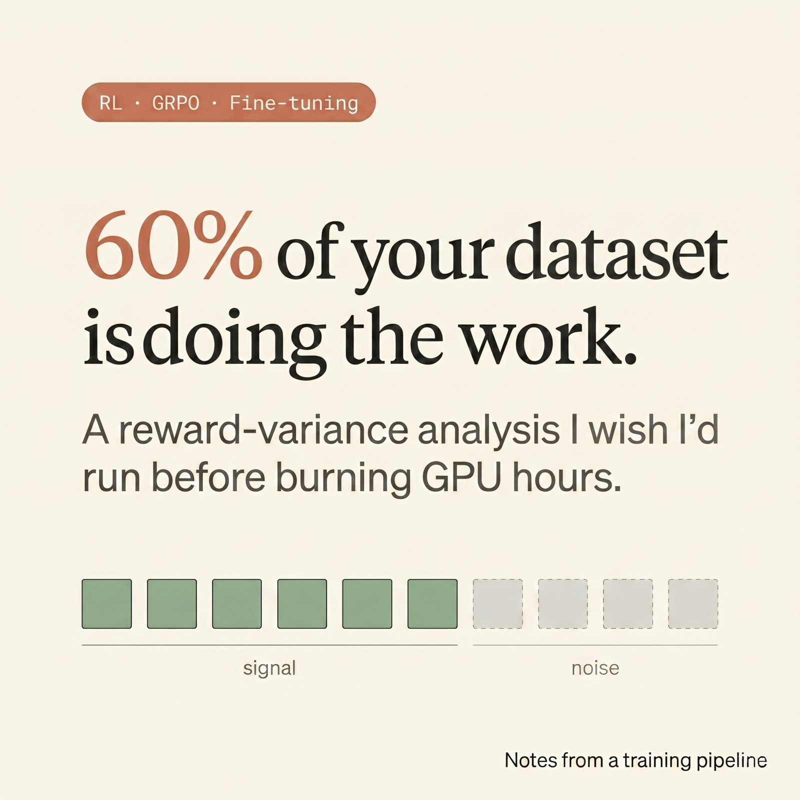
60% of your dataset is doing the work — a GRPO reward-variance analysis

A mistake I made early in my training pipeline: I assumed my curated dataset was my dataset.

TL;DR — GRPO learns from how much the rollouts inside a group disagree with each other. When all rollouts agree (all pass, or all fail), there's nothing to compare, so the model doesn't update. On a typical "curated" dataset, a meaningful fraction of prompts produce these silent dead-weight groups. A 30-minute pre-flight check tells you exactly which prompts are actually teaching your model and which are just running up the GPU bill.

The setup

I was running GRPO fine-tuning on a reasoning model. The training metrics looked, by every reasonable indicator, healthy. The loss curve trended down smoothly. Mean reward across rollouts trended up. KL against the reference model was within bounds. Group-relative advantages had the right distribution shape.

Eval told a different story. Pass-rate uplift on the held-out set was embarrassingly small for the compute I'd burned. Not flat — there was improvement — but the slope-to-cost ratio was wrong. I'd seen the same recipe land much better on prior runs with smaller datasets.

The first instinct in this situation is to reach for hyperparameters. Try a different KL coefficient. Lower the learning rate. Increase clip range. I almost did that. Instead I stopped training and ran the analysis I should've run on day one — a reward / policy diagnostic on the base model, before a single gradient step.

The result: roughly 40% of my carefully curated dataset was producing exactly zero learning signal. It looked like training data on disk. It wasn't training data in any operational sense.

What GRPO is actually doing

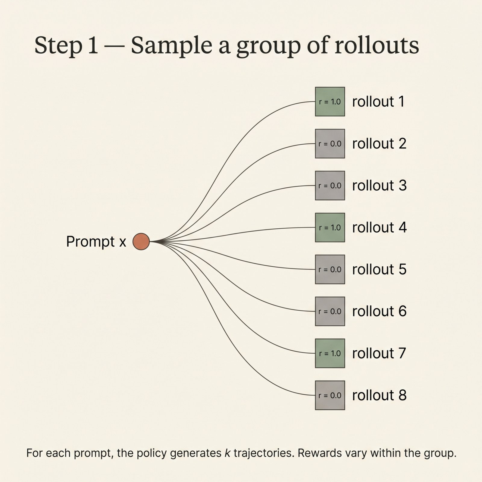
Imagine you give the same exam question to four students from the same class. They all hand in different answers. Two get it right, two get it wrong. As a teacher, you can compare them and say "do more of what the first two did, less of what the other two did." That's a useful lesson because the four answers differed.

Now imagine you give the same question to four students and all four hand in identical answers. There's nothing to compare. You can't tell which version was better. There's no lesson.

That's GRPO. For each prompt, it samples k rollouts from the model (the "students"), scores each rollout, and the training signal is the difference between rollouts inside the same group. No difference, no lesson.

For each prompt's group of k rollouts, GRPO normalises the rewards into "advantages":

# Pseudocode for a single prompt's group
rewards = [reward(rollout_i) for rollout_i in rollouts]   # k values
mu = mean(rewards)
sigma = std(rewards)
advantages = [(r - mu) / (sigma + eps) for r in rewards]

The training objective is then a clipped policy gradient weighted by these per-rollout advantages, plus a KL penalty against a reference model. There's no value network — the value head PPO relies on for advantage estimation is gone. The signal you're optimising against comes entirely from how much the rollouts inside one group disagree.

This is great when it works. You drop a whole component (the value head), simplify the loop, sidestep the value-bias problem, and get a clean objective. The catch is hiding in plain sight in that division by sigma.

The trap: when the group agrees

Suppose for some prompt, all k rollouts get the same reward. Maybe the model already solves the problem reliably and every rollout passes. Maybe it can't solve it at all and every rollout fails. Either way:

• The mean reward equals every individual reward.
• Standard deviation (σ) is zero.
• Every rollout's advantage is zero.
• The lesson the model takes away from that prompt is: nothing.

You still pay the full cost. K rollouts of inference. Forward and backward passes through the actor. Forward pass through the reference model on every token. All of it produces a gradient term of exactly zero for that prompt.

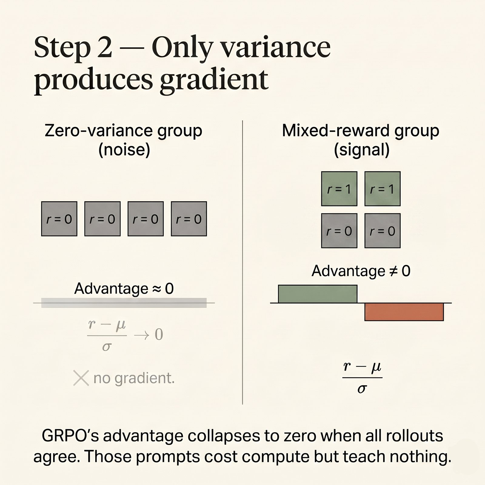
If you've ever stared at a training run and thought "the loss is moving but the model isn't really getting better at the underlying task" — this is one mechanism that produces that exact pattern. Zero-variance groups don't crash training; they silently dilute it. Your effective batch size shrinks without any signal that it's happening.

Worked example: tool use, end to end

The mechanics are easier to see on a concrete tool-calling task. Suppose the model has access to two tools:

convert_currency(amount: float, from_currency: str, to_currency: str) -> float
web_search(query: str) -> str

And we ask it:

Prompt x: "What's 500 USD in Indian rupees today?"

The verifier is simple and binary. The answer is correct if it's within ±2% of the true conversion (let's call that ₹41,750), produced via a valid convert_currency call. Anything else fails.

Sample k = 4 rollouts from the current policy:

Rollout y₁ — picks the right tool, right parameters

<think>I'll convert 500 USD to INR using the currency tool.</think>
<tool_call>convert_currency(amount=500, from_currency="USD", to_currency="INR")</tool_call>
<observation>41750.0</observation>
500 USD ≈ ₹41,750.

Verifier: ✓ → r₁ = 1.0

Rollout y₂ — wrong tool entirely

<think>Let me search for the current rate.</think>
<tool_call>web_search(query="500 dollars to rupees")</tool_call>
<observation>"As of last year, 1 USD ≈ ₹83. Rates fluctuate daily..."</observation>
500 USD is around ₹40,000 today.

Verifier: ✗ (wrong tool, answer also outside tolerance) → r₂ = 0.0

Rollout y₃ — right tool, right parameters, slightly different style

<tool_call>convert_currency(500, "USD", "INR")</tool_call>
<observation>41750.0</observation>
That's about ₹41,750 — roughly ₹83.50 per dollar.

Verifier: ✓ → r₃ = 1.0

Rollout y₄ — right tool, wrong parameters (swapped direction)

<tool_call>convert_currency(amount=500, from_currency="INR", to_currency="USD")</tool_call>
<observation>5.99</observation>
That comes out to about ₹6.

Verifier: ✗ (parameters reversed → wrong amount) → r₄ = 0.0

Group statistics: μ = 0.5, σ = 0.5 (population std, the n-divisor convention used by most GRPO implementations including the default torch.std(..., unbiased=False) path). Advantages, computed as Aᵢ = (rᵢ − μ) / σ:

A₁ = +1.0   (rollout 1, passed)
A₂ = −1.0   (rollout 2, failed)
A₃ = +1.0   (rollout 3, passed)
A₄ = −1.0   (rollout 4, failed)

(If your trainer uses sample std with the n−1 divisor, σ ≈ 0.577 here and advantages are ±0.87. Same direction, slightly smaller magnitude.)

What the model actually learns from this group

The training step looks at all four rollouts at once. It tells the model:

• Do more of what y₁ did. Calling convert_currency with USD and INR in the right slots, then phrasing the answer cleanly. Every token in y₁ — including the tool name and the argument values — has its log-probability nudged up by 1.0.
• Do more of what y₃ did. Same shape as y₁, slightly different style. Also nudged up by 1.0.
• Do less of what y₂ did. Reaching for web_search when a structured tool exists. Every token in y₂, including the wrong tool name, gets nudged down by 1.0.
• Do less of what y₄ did. Calling the right tool but with the wrong argument order — INR and USD swapped. Those specific tokens get nudged down. The model isn't learning "tool calls are bad". It's learning "this exact swapped argument shape is bad".

The policy-gradient term for this prompt is:

∇_θ L  =  Σᵢ Aᵢ · ∇_θ log πθ(yᵢ | x)

(plus clipping and a KL penalty against the reference, which we'll skip for the intuition). The per-token weight is the advantage. Positive advantage → log-probability of every token in that rollout goes up. Negative → it goes down.

So when someone asks "which rollout uplifted the policy?" — the honest answer is all four did — in opposite directions. The training signal lives in the spread between rollouts inside the group, which is exactly why the spread has to be non-zero for anything to happen.

Aside: real reward functions are usually decomposed

In production tool-use training, the reward usually isn't a single binary. It's typically a sum of finer signals — for example:

R_total = R_format     # did the tool call parse as valid JSON?
        + R_tool_choice  # did the model pick a tool that could plausibly answer?
        + R_param_match  # do the args satisfy the tool's schema and look right?
        + R_outcome      # did the final answer pass the end-to-end verifier?

This gives the policy partial credit. y₄ above would now score something like R_format=1, R_tool_choice=1, R_param_match=0.5, R_outcome=0. That's more signal than a flat 0/1 — the model gets to learn "your tool choice was right, your parameters weren't" instead of just "you failed". As a side effect, denser reward landscapes tend to produce more signal-bucket prompts (more on that below), because edge cases that would tie at 0 or 1 with a binary reward now get spread across the middle.

Now collapse the variance

Imagine instead that all four rollouts had passed, or all four had failed. Same k = 4, same forward and backward passes through the actor and reference model — but now μ equals every reward, σ = 0, and every Aᵢ = 0. The lesson term is the zero vector. The policy moves nowhere.

You paid for the compute. You got no learning. That's the trap, and the next section is how to spot it before you waste a training run on it.

The bridge: your base model's average tells you the bucket sizes

Here's the connection a lot of people skip.

Your base model has some overall pass rate on your dataset — let's say 0.67. That number is the average across all prompts and all rollouts. It does not mean that 67% of every prompt's rollouts pass.

Within that 0.67 average, individual prompts split into very different shapes:

• Some prompts the model always passes. Pass rate per prompt = 1.0.
• Some prompts the model never passes. Pass rate per prompt = 0.0.
• Some prompts the model sometimes passes. Pass rate per prompt is somewhere in between.

The aggregate hides the buckets. A dataset where every prompt sits at 0.67 pass-rate looks identical to a dataset where 67% of prompts sit at 1.0 and 33% sit at 0.0 — same average, completely different training behaviour.

For GRPO, only the third bucket — prompts where the model sometimes passes and sometimes fails — actually teaches anything. The other two are dead weight no matter how high your overall average looks.

So the real question for any dataset isn't "what's my base model's average reward?" It's "how many of my prompts are in the third bucket?"

The pre-flight check

The fix is a one-pass diagnostic on the base model, before the first GRPO step. The idea: run the base model on every prompt a few times, see how often it succeeds, and sort prompts into the three buckets above.

# Pre-flight reward-variance sweep on base policy
K = 16  # rollouts per prompt for estimation
buckets = {"unlearnable": [], "trivial": [], "signal": []}
 
for prompt in dataset:
    rollouts = [base_policy.generate(prompt) for _ in range(K)]
    rewards = [verifier(prompt, r) for r in rollouts]   # 0/1 or graded
    pass_rate = sum(rewards) / len(rewards)
 
    if pass_rate == 0.0:
        buckets["unlearnable"].append(prompt)
    elif pass_rate == 1.0:
        buckets["trivial"].append(prompt)
    else:
        buckets["signal"].append(prompt)
 
print({k: len(v) for k, v in buckets.items()})

Three buckets, three different problems:

• pass_rate == 0 — the model can't solve this at all right now. Every rollout fails, so within-group variance is zero, and GRPO learns nothing. Could become learnable later if the policy improves enough to occasionally succeed, but right now it's dead weight. In the worst case it's also out-of-distribution noise.
• pass_rate == 1 — the model already solves this reliably. Variance is zero on the other end. The policy has nothing left to learn from this prompt; you'd just be reinforcing what it already does.
• 0 < pass_rate < 1 — the model sometimes succeeds. There's spread inside the group. The lesson exists. Gradient flows.

Only the third bucket trains anything. The other two cost you GPU hours.

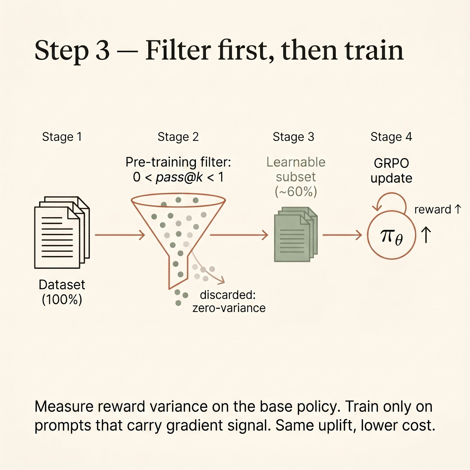
What I found

When I ran the sweep on what I'd been treating as my training set, the split surprised me. About 60% of prompts landed in the signal bucket. The other 40% split between unlearnable (the larger half — the base model couldn't solve them at all) and trivial (already solved). I'd been paying full GRPO cost on every one of them.

I filtered to the signal-carrying subset, re-ran GRPO at the same hyperparameters and same compute budget, and got two things:

1. Same eval uplift, lower cost. When I matched the original training run's eval delta, I'd burned meaningfully fewer GPU-hours. Every step now had non-zero contribution.
2. Stronger policy at the same budget. When I matched the original compute budget instead, the policy ended up better. Same forward and backward passes, but every one of them was carrying a real lesson.

The headline framing — "60% of your dataset is doing the work" — wasn't a metaphor. It was the entire optimisation story. The remaining 40% wasn't training the model, it was just inflating the bill.

How many rollouts to use for the sweep

The sweep itself is a noisy estimate. With only k = 8 rollouts per prompt, a prompt that has a true 5% pass rate has roughly a 66% chance of looking like pass_rate == 0 in your sweep. You'd misclassify it as unlearnable when it's actually a borderline signal-bucket prompt.

Practical guidance:

• k = 16 for the sweep. It's a one-time cost and the higher k buys you better estimates of the rare-but-real pass rates at the tails.
• k = 8 during actual training. The group size during the GRPO loop is a separate decision driven by compute and gradient noise, not by the filtering accuracy.
• Soft thresholds at the edges. Instead of pass_rate == 0 and pass_rate == 1, try pass_rate < 0.05 and pass_rate > 0.95. This rescues borderline prompts and avoids over-aggressive filtering.

When this approach goes wrong

A few cases where straight variance filtering will steer you wrong:

• Curriculum learning is intentional. If your plan is to train on increasingly hard prompts as the policy improves, today's pass_rate == 0 is tomorrow's signal bucket. Run the sweep periodically (e.g. every N training steps) and re-bucket — don't filter once and lock it in.
• Rare-but-important prompts. Some unlearnable prompts represent failure modes you genuinely care about — security-critical refusals, edge-case correctness. Filtering them out improves training efficiency and removes pressure on those failure modes. Keep them in a separate eval, not in the training mix.
• Reward sparsity. If your reward function is so harsh that almost every prompt sits at pass_rate == 0, the problem is upstream — your reward design, not your data. Reward shaping or process rewards may help; variance filtering won't, because there's no variance anywhere.
• Off-policy drift. The sweep estimates variance under the base policy. As GRPO trains, the policy moves, and the variance distribution shifts. A prompt that was zero-variance at step 0 may become signal-bucket at step 1,000 (and vice versa). Re-running the sweep mid-training is cheap insurance.

A reproducible recipe

If you're about to run GRPO on your own dataset, here's the minimum-viable version of this analysis:

1. Pick K between 8 and 16 for the sweep.
2. For each prompt in your training set, generate K rollouts from the base (pre-RL) policy and score them with the same verifier you'll use during training.
3. Bucket prompts by pass rate. Use hard thresholds initially (== 0, == 1, otherwise) to get a feel for the distribution; consider soft thresholds if you have lots of prompts at the extremes.
4. Plot the pass-rate histogram. The shape tells you whether you have a data problem, a reward problem, or a reward-too-sparse / reward-too-loose problem.
5. Train GRPO on the signal bucket only.
6. Re-run the sweep every few hundred steps. Re-bucket. Repeat.

The whole thing is one script and a few hours of inference. The cost is negligible compared to a real training run, and it tells you exactly where your compute is going.

The takeaway

GRPO's elegance is that the group baseline removes a whole class of bias — but it pushes the data-quality problem squarely onto the dataset itself. The objective is honest: it tells you that prompts without within-group variance contribute nothing to the gradient. Most "curated" datasets aren't.

Your effective dataset is smaller than you think. The gap between "curated" and "learnable" is where most of your compute quietly dies. Measure the gap before you scale.